Project C1 • Local inversion for linear seismic imaging
Principal investigators
apl. Prof. Dr. Peer Kunstmann
(7/2015 - )
Prof. Dr. Andreas Rieder
(7/2015 - )
Project summary
In this project we reconstruct subsurface material parameters, for example under the earth's or the ocean's surface. To this end, sources on the surface excite pressure waves going through the material below. Then, the geological inner structure scatters these waves and those parts returning to the surface are recorded by receivers. By using these measurements we image these material parameters.
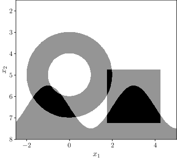
Figure 1. Fabricated subsurface structure (left), and corresponding reconstructions from ideal generated data (middle) or from data of a wave solver (right).
Here, the subsurface materials are determined by their wave speed $\nu_{\mathrm{pr}} = \nu_{\mathrm{pr}}(\boldsymbol x)$. If a source is excited at time $t = 0$ and location $\boldsymbol{x_s}$, then the resulting pressure wave $u(t; \boldsymbol{x}, \boldsymbol{x_s})$ traveling through the material is described by the acoustic wave equation \begin{equation}\label{eq:wave_eq} \frac{1}{\nu_\mathrm{pr}^2} \partial_t^2 u - \Delta u = \delta(\boldsymbol{x} - \boldsymbol{x_s})\delta(t), \quad u\vert_{t=0} = \partial_t u\vert_{t=0} = 0. \end{equation} Thus, for a receiver at position $\boldsymbol{x_r}$, the recorded measurements are $u(t; \boldsymbol{x_r}, \boldsymbol{x_s})$. Our aim now is to reconstruct $\nu_{\mathrm{pr}}$ from those measurements.
In a first step, the sought-for quantity $\nu_{\mathrm{pr}}$ is replaced by an equivalent quantity $n$ which, in contrast to $\nu_{\mathrm{pr}}$, is described by a linear parameter identification problem \begin{equation*} F n = g \end{equation*} for some operator $F$ and right-hand side $g$ based on the measurements, see details below. The problem of obtaining $n$ from $g$ is the linearized inverse problem of seismic imaging.
A further challenge is that there is no inversion formula for $F$. Therefore, instead of reconstructing $n$ directly, we reconstruct certain important properties of $n$, especially jumps, by developing, analyzing and testing a migration scheme based on designed imaging operators in two (and three) dimensions.
Let $c$ be a smooth and known background wave speed satisfying the geometric optics approximation, that is, no multiple reflections or caustics occur. By using the linearization ansatz \begin{equation*} \frac{1}{\nu_\mathrm{pr}^2(\boldsymbol{x})} = \frac{1+n(\boldsymbol{x})}{c^2(\boldsymbol{x})}, \end{equation*} where $\boldsymbol{x}\in\mathbb{R}^d$ with spatial dimension $d\in\{2,3\}$, the now sought-for quantity $n$ is a dimensionless reflectivity capturing the high frequency variations, i.e. jumps, of the true wave speed $\nu_\mathrm{pr}$.
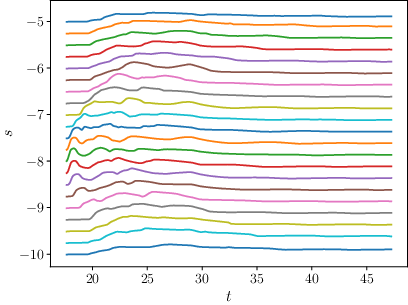
The linearized inverse problem of seismic imaging entails solving \begin{equation}\label{eqn_for_n} Fn(t; \boldsymbol{x_r}, \boldsymbol{x_s}) = g(t; \boldsymbol{x_r}, \boldsymbol{x_s}) \end{equation} for $n$, where $g$ are pre-processed seismic measurements for several instants of time $t$ and for several source positions $\boldsymbol{x_s}$ and receiver positions $\boldsymbol{x_r}$ (see Figure 2).
Figure 2. Example for processed data $g$ (in this case from a wave solver). Every line corresponds to one receiver position and is scaled appropriately.
The involved operator \begin{equation}\label{eq:genRadon} F w(t, \boldsymbol{x_r}, \boldsymbol{x_s}) = \int \frac{w(\boldsymbol{x})}{c^2(\boldsymbol{x})} a(\boldsymbol{x}, \boldsymbol{x_s}) a(\boldsymbol{x_r},\boldsymbol{x})\; \delta\left(t - \tau(\boldsymbol{x}, \boldsymbol{x_s}) - \tau(\boldsymbol{x}, \boldsymbol{x_r})\right)\, \mathrm{d}\boldsymbol{x} \end{equation} is a generalized Radon transform (GRT) in which the travel time $\tau$ and the amplitude $a$ solve the eikonal equation \begin{equation*} \lvert \nabla \tau(\cdot, \boldsymbol{x_s})\rvert^2 = \frac{1}{c^2(\cdot)},\quad \tau(\boldsymbol{x_s}, \boldsymbol{x_s}) = 0, \end{equation*} and the transport equation \begin{equation*} 2 \nabla a(\cdot, \boldsymbol{x_s}) \cdot \nabla \tau(\cdot, \boldsymbol{x_s}) + a(\cdot, \boldsymbol{x_s}) \Delta \tau(\cdot, \boldsymbol{x_s}) = 0. \end{equation*} The processed data $g$ of \eqref{eqn_for_n} are given by \begin{equation*} g(t, \boldsymbol{x_r}, \boldsymbol{x_s}) = 4\pi \int_0^t (t-r)^{d-2}(\widetilde{u} - u)(r; \boldsymbol{x_r},\boldsymbol{x_s})\, \mathrm{d}r, \end{equation*} where $d\in\{2,3\}$ is the spatial dimension, $u$ are the recorded seismic measurements (reflected wave field) and \(\widetilde{u}\) is the computed reference solution of eq. \eqref{eq:wave_eq} with $\nu_{\mathrm{pr}}$ replaced by $c$.
In the following, we restrict ourselves to two spatial dimensions. However, we obtained similar results for the three dimensional situation [GKQR18b].
We work under the following assumptions.
The background velocity $c$ is layered, meaning it depends only on the depth coordinate ($c(\boldsymbol{x}) = c(x_2)$).
Further, with $X = \mathbb{R}^2_+ = \{\boldsymbol{x}=(x_1,x_2)^\top \in \mathbb{R}^2\,\vert\, x_2 > 0\}$ we consider $n\in L^2(X)$ with compact support.
We use the common offset data acquisition geometry with offset $\alpha \ge 0$, where sources and receivers are parameterized by $s \in \mathbb{R}$ via \begin{equation*} \boldsymbol{x_s}(s) = (s-\alpha,0)^\top \quad\text{and}\quad \boldsymbol{x_r}(s)=(s+\alpha,0)^\top. \end{equation*}
Thus, the 2D generalized Radon transform \eqref{eq:genRadon} may be written as \begin{equation*} \begin{aligned} Fn(s,t) &= \int_X A(s,\boldsymbol{x}) n(\boldsymbol{x})\; \delta\left(t - \varphi(s, \boldsymbol{x})\right)\, \mathrm{d}\boldsymbol{x}&\\ &= \int_{\mathfrak{L}(s, t)} \frac{A(s,\boldsymbol{x}) n(\boldsymbol{x})}{\lvert \nabla \varphi(s, \boldsymbol{x})\rvert}\, \mathrm{ds}(\boldsymbol{x}) ,\quad &t \geq t_\text{first}, \end{aligned} \end{equation*} with \begin{equation*} \varphi(s, \boldsymbol{x})≔ \tau(\boldsymbol{x}, \boldsymbol{x_s}(s)) + \tau(\boldsymbol{x}, \boldsymbol{x_r}(s)) \quad\text{and}\quad A(s, \boldsymbol{x}) = \frac{a(\boldsymbol{x}, \boldsymbol{x_s}) a(\boldsymbol{x}, \boldsymbol{x_r})}{c^2(\boldsymbol{x})}. \end{equation*} Here, $t_\text{first} = t_\text{first}(s)$ is the first arrival time, that is, the minimal time a wave needs to travel from source to receiver. The GRT integrates over the reflection isochrones $\mathfrak{L}(s, t)≔ \{\boldsymbol{x}\in X \colon \varphi(s, \boldsymbol{x}) = t\}$.
Further, let $S_0\subset\mathbb{R}$ be the bounded open set containing the parameters for the source receiver pairs. For this setting we introduce an imaging operator.
Our imaging operator
Under the assumptions above we consider the linearized inverse problem \eqref{eqn_for_n} on the data space $Y=S_0\times \lbrack t_\text{first}, \infty\lbrack$. Here, we do not try to reconstruct $n$ directly (there is no inversion formula in general, even in the full data case, $S_0=\mathbb{R}$). Instead, we define imaging operators of the form \begin{equation}\label{imaging_op} \Lambda:=K F^\dagger \Psi F, \end{equation} where $\Psi\colon Y\to \lbrack 0, \infty\lbrack$ is a smooth compactly supported cutoff function and $K$ is a properly supported pseudodifferential operator on $X$ of non-negative order $\kappa$. Further, $F^\dagger$ is the generalized backprojection operator \begin{equation*} F^\dagger u(\boldsymbol{x})= \int_{S_0} W(s, \boldsymbol{x}) u(s, \varphi(s, \boldsymbol{x}))\, \mathrm{d} s \end{equation*} for $u\in\mathfrak{D}(Y)$, where $W$ is a smooth positive weight. Then, the composition $F^\dagger\Psi F$ is well-defined for distributions with compact support. Note that the formal $L^2$-adjoint $F^*$ has the weight $W=A$.
Motivation and Results for explicit choices of \(\Lambda\)
Our imaging operator $\Lambda$ is a pseudodifferential operator of order $\kappa - 1$. Thus, the reconstruction \begin{equation*} \Lambda n=KF^\dagger\Psi g \end{equation*} from measured data $g$ (in an ideal setting: $g=Fn$) shows some singularities of $n$. The cutoff $\Psi$ adds no non-smooth artifacts, so it has no influence on the singularities. For these reasons we chose $\Lambda$ as in \eqref{imaging_op}. In directions where $\Lambda$ is microlocally elliptic the singularities are even emphasized. To study its (microlocal) ellipticity we computed the top order symbol of $\Lambda$.
Our first choice $F^\dagger=F^\ast$ and $K=\Delta$ with the Laplacian $\Delta$ resulted in an operator $\Lambda$ of order $1$. Further studies of the symbol led us to choose $F^\dagger = F^*$ and $K=\Delta (M^q +\beta\operatorname{Id})$ with $M$ being the multiplication operator by $x_2$, and $\beta, q \geq 0$ suitable constants. This operator, also of order $1$, reconstructs jumps in $n$ having the same height but being located at different depths with the same intensities almost independent of the offset $\alpha$.
Stability with respect to sound speed
Our results use in an essential way that certain Fourier integral operators, that are part of the imaging operator $\Lambda$, are actually pseudodifferential operators, which therefore map singularities in a favorable way. We showed in [KQR22] that this property is stable under small and sufficiently smooth variations of the wave speed. This means that our general abstract results persist to hold for wave speeds that are small smooth perturbations of a constant or a linearly increasing wave speed.
Numerical experiments: Method of the approximate inverse
The structure of $\Lambda$ suggest to use the concept of approximate inverse for imaging. This means, we calculate a smoothed version of $\Lambda n$ by using duality arguments.
Let $\{e_{\gamma}\}_{\gamma > 0}$ be a family of mollifiers, that is, $e_\gamma\to\delta$ as $\gamma \to 0$. Further, let $e_{\gamma}$ be compactly supported in the ball about the origin with radius $\gamma$. Then, for $\boldsymbol{p} = (p_1, p_2)^\top\in X$ and $0 < \gamma < p_2$, we have \begin{equation*} \Lambda n \ast e_\gamma (\boldsymbol{p})= \langle \Psi g, v_{\boldsymbol{p},\gamma}\rangle_{L^2(Y)}\quad\text{for } g=Fn \end{equation*} where the reconstruction kernel $v_{\boldsymbol{p}, \gamma}$ is given by \begin{equation*} v_{\boldsymbol{p},\gamma} = F K^* e_{\gamma}(\,\cdot\, - \boldsymbol{p}). \end{equation*}
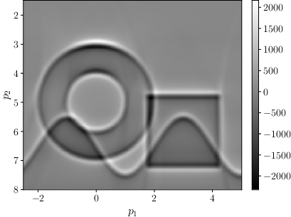
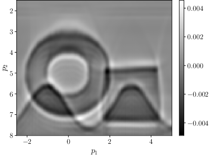
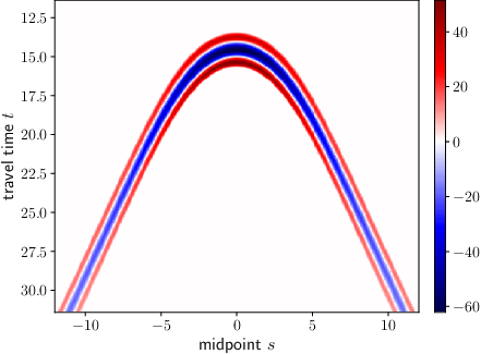
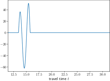
Figure 3. Reconstruction kernel $v_{(0, 4), 0.8}$ for $K = \Delta M^2$. The cross section on the right is taken for $s=0$.
We calculated the reconstruction kernel for a certain family of mollifiers numerically. So, by taking the inner product with the data $g$ we get the smoothed version $\Lambda n \ast e_\gamma (\boldsymbol{p})$ of $\Lambda n(\boldsymbol{p})$.
An example kernel and reconstructions for a linear velocity model $c(\boldsymbol{x}) = 0.1 x_2 + 0.5$ can be seen in Figure 3 and Figure 1. We used a phantom $n=\chi_{B_2((0,5), 2)} - \chi_{B_2((0,5), 1)} + \chi_{B_\infty((3,6), 1.25)} + \chi_{x_2 \ge 6.5+\sin(\pi x_1 / 2)}$ (left in Figure 1) to generate our data. For the reconstructions we used ideal data calculated by applying $F$ to $n$ (middle of Figure 1), and also data $g$ obtained from a wave solver for a suitable real velocity $\nu_\mathrm{pr}$ (right of Figure 1).
For more details and the implementation of the scheme, see [GR22]. The results from the figures above were obtained using our software package [G22]. Continue reading.Collapse content.