Project A12 • Dynamics of the Gross–Pitaevskii equation and related dispersive equations
Principal investigators
JProf. Dr. Xian Liao
(1/2020 - )
Prof. Dr. Guido Schneider
(1/2020 - )
Project summary
The one-dimensional Gross-Pitaevskii (GP) equation \begin{equation}\label{GP} \tag{GP} i \partial_t q + \partial_{xx} q = 2 (|q|^2 - 1) q, \qquad t, x \in \mathbb{R}, \qquad q = q(t, x): \mathbb{R} \times \mathbb{R} \rightarrow \mathbb{C} \end{equation} is a prototypical model in many fields, such as Bose-Einstein condensation, deep water waves and nonlinear optics. Here the wave function $q$ satisfies the following nonzero boundary condition at infinity \begin{equation}\label{NZBC} \tag{NZBC} |q(t, x)| \rightarrow 1, \quad |x| \rightarrow \infty, \end{equation} which is of great physical interest, e.g. it corresponds to the propagation of waves through a condensate of constant density in the context of Bose-Einstein condensation. This \eqref{NZBC} drastically changes the dynamics from the closely related defocusing cubic nonlinear Schrödinger \eqref{NLS} equation \begin{equation}\label{NLS} \tag{NLS} i \partial_t \psi + \partial_{xx} \psi = 2|\psi|^2 \psi, \qquad t, x \in \mathbb{R}, \qquad \psi = \psi(t, x): \mathbb{R} \times \mathbb{R} \rightarrow \mathbb{C}, \end{equation} whose solution $\psi$ satisfies the zero boundary condition \begin{equation}\label{ZBC} \tag{ZBC} |\psi(t, x)| \rightarrow 0, \quad |x| \rightarrow \infty. \end{equation}
For \eqref{NLS}-\eqref{ZBC} there are (modified) scattering results, and the solutions spread out and decay for large times. Contrary to this, \eqref{GP}-\eqref{NZBC} possesses a family of soliton solutions $(q_c)_{c\in (-1,1)}$, and for each $c\in (-1,1)$, $q_c$ reads explicitly \begin{equation}\tag{Qc}\label{Qc} q_c(t, x) = Q_c(x - 2 c t) \quad \text{ with } \quad Q_c(x) = \sqrt{1 - c^2} \tanh(\sqrt{1 - c^2} x) + i c. \end{equation}
Left: The wave front of the dark soliton as the speed $c$ ranges from $-1$ to $1$, viewed in a co-moving frame. Center: The range of the dark soliton as a subset of the complex plane. Right: The squared magnitude of the dark soliton.
The word soliton is a combination of the terms solitary wave and particle. It describes (localized) traveling waves that exhibit some particle-like behavior, such as stability under perturbations or interaction with other solitons.
If $c=0$, then $q_0(t,x)=\tanh(x)$ denotes the (time-independent) black soliton, with the (light) density $|q_0|^2=1-{\text{sech}}^2(x)$ vanishing at the origin, which heuristically corresponds to the black point in nonlinear optics. If $c\in (-1,0)$ or $(0,1)$, then the dark solitons $q_c$ travels to the right or to the left at the constant speed $2|c|<2$, with a kink in the density function $|q_c|^2$ at the point $x=2ct$, which heuristically corresponds to the dark point in nonlinear optics. There are no soliton solutions travelling faster than the speed $2$.
The interesting dynamics of \eqref{GP}-\eqref{NZBC} are not yet well understood, since the dispersion effect is weak in dimension one and the analytical framework for functions with nonzero boundary conditions is more delicate. The first aim of this project is to develop tailor-made analysis tools to study the dynamics of \eqref{GP}-\eqref{NZBC} in the well-established analytical framework. The second aim of this project is to extend the analytical tools and results for \eqref{GP}-\eqref{NZBC} to other related dispersive equations, such as the complex cubic Klein–Gordon \eqref{ccKG} equation or the Korteweg–de Vries (KdV) equation.
Analytical Framework for (GP)
The conserved Ginzburg-Landau energy of the \eqref{GP} equation reads as \begin{equation*} E(q)=\int_{\mathbb{R}}\Bigl( \bigl(|q|^2-1\bigr)^2+|\partial_x q|^2\Bigr)\,\mathrm{d}x=\|(|q|^2-1, \partial_xq)\|_{L^2(\mathbb{R})}^2. \end{equation*} This motivates us to consider generalized finite-energy functions in the following space: \begin{equation}\tag{Xs}\label{Xs} X^s=\bigl\{q\in H^s_{\textrm{loc}}(\mathbb{R}; \mathbb{C})\,|\, E^s(q):=\|( |q|^2-1, \partial_xq)\|_{ H^{s-1}(\mathbb{R})}^2 <\infty\bigr \}/{\mathbb{S}^1}, \quad s\geq 0. \end{equation} Continue reading: More explanations on the defintion of $X^s$.Collapse content.
Due to \eqref{NZBC}, the usual functional framework such as Sobolev spaces are not suitable for the solutions of \eqref{GP} anymore. We consider the tailor-made solution spaces $X^s$ for \eqref{GP}:
The module of the unit circle $\mathbb{S}^1$ is motivated by the $\mathbb{S}^1-$symmetry of \eqref{GP};
The constant functions $1=-1=i=-i$ are the same element in $X^s$, and have zero energy ${E}(1)=0$;
$X^s$ is not a vector space;
The soliton solutions $q_c(t,\cdot)\in X^s$ since \begin{align*} -(|q_c(t,x)|^2-1)=(1-c^2)\text{sech}^2\bigl(\sqrt{1-c^2}(x-2ct)\bigr)=\partial_x q_c(t,x); \end{align*}
The finite-energy function $q\in X^s$ satisfies the nonzero boundary condition \eqref{NZBC} in the sense that $|q|^2-1\in H^{s-1}(\mathbb{R})$;
If $s=1$, $X^1$ denotes the (classical) energy space \begin{equation*} X^1=\bigl\{q\in H^1_{\textrm{loc}}(\mathbb{R}; \mathbb{C})\,|\, E(q)=\|( |q|^2-1, \partial_xq)\|_{ L^2(\mathbb{R})}^2 <\infty\bigr \}/{\mathbb{S}^1}. \end{equation*}
We equip the space $X^s$ with the distance function \begin{equation}\tag{ds}\label{ds} d^s(q, p) = \left( \int_{\mathbb{R}} \inf_{|\lambda| = 1} \|\text{sech}(y - \cdot) (\lambda q - p)\|_{H^s(\mathbb{R})}^2 \right)^{\frac12}\,, \end{equation} such that $(X^s, d^s)$ is a complete metric space. The analytic and the topological structures of $(X^s, d^s)$ are highly nontrivial ([KL21, KL22]). Continue reading: More explanations on the metric space $(X^s,d^s)$.Collapse content.
The distance function $d^s(q,p)$ measures the differences between $q$ and $p$ in a nonlinear way:
Because the integral in (ds) contains an infimum over phase rotations $\lambda \in \mathbb{S}^1$, it is possible for two functions $q, p$ to have different asymptotic phases at infinity while having a finite distance $d^s(q, p)$. This makes $(X^s, d^s)$ a natural space for functions with \eqref{NZBC};
The distance $d^s(q,1)$ is (locally) equivalent to the energy $E^s(q)=\|( |q|^2-1, \partial_xq)\|_{ H^{s-1}(\mathbb{R})}^2$;
For $s > \frac12$ and two (nowhere vanishing) functions $q = \sqrt{\rho} e^{i \phi}, p = \sqrt{\eta} e^{i \psi} \in H_{\textrm{loc}}^s(\mathbb{R})$, $d^s(q,p)$ is (locally) equivalent to both \begin{align*} \sum_{k \in \mathbb{Z}} \inf_{|\lambda| = 1} \|\lambda q - p\|_{W^{s,2}(\{x \in \mathbb{R}: \,|x - k| \leq 1\})} \end{align*} and \begin{align*} \theta^s((\rho, v), (\eta, w)) = \|\rho - \eta\|_{H^s(\mathbb{R})} + \|v - w\|_{H^{s-1}(\mathbb{R})} \,, \end{align*} where $v,w$ denote the phase velocities $\partial_x\varphi, \partial_x \psi$ respectively;
$1+\mathcal{S}(\mathbb{R})$ is dense in $(X^s, d^s)$;
The set of $1$ and the soliton profiles $\{Q_c: c \in [-1,1] \}$ is a strong deformation retract of $(X^s, d^s)$, and hence $X^s$ is homotopy equivalent to a circle;
Complete Integrability and Global-in-time Wellposedness of (GP)
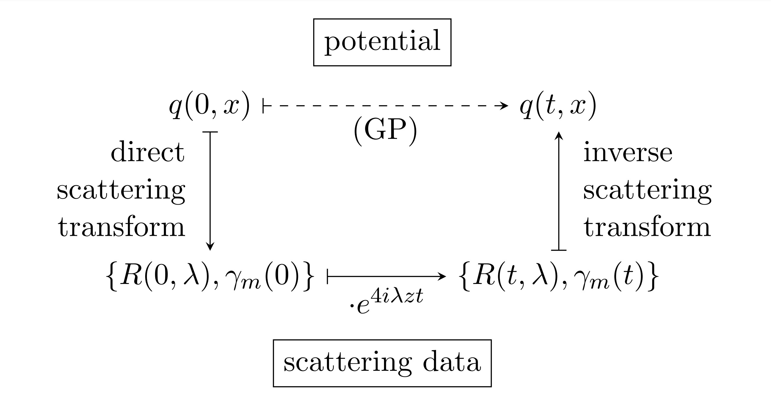
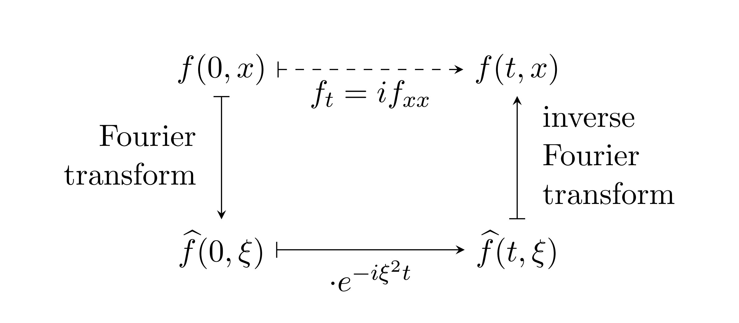
The Gross-Pitaevskii equations are completely integrable. In the broad sense, this means that they have a high rigidity that makes it possible to explicitly write down solutions using integrals. In our case, it means that the Gross-Pitaevskii flow, which is a nonlinear time-evolution of the initial data, can be transformed to a linear evolution of the \emph{scattering data} associated to the problem. Similarly to the method of solving linear equations via the Fourier transform, the solution to the problem can be recovered by the scattering data by the inverse scattering transform:
Compare this to the method of solving the Schrödinger equation $i f_t + f_{xx} = 0$ via the Fourier transform:
Leveraging this integrable structure is central to the analysis of the \eqref{GP} equation, and as a result there are deep connections between \eqref{GP} and other integrable systems.
The scattering data is related to the spectral problem of the so-called Lax operator of \eqref{GP} \begin{equation}\tag{Lax}\label{Lax} L = \begin{pmatrix} i \partial_x & - i q \\ i \overline{q} & i \partial_x \end{pmatrix}\,. \end{equation} Contrary to the time evolution of the scattering data, the spectrum of $L$ as well as the transmission coefficient $T^{-1}(\lambda)$ are time-independent. The conservation of the transmission coefficient implies the existence of a family of conserved quantities. From these one obtains uniform-in-time bounds for the energy $E^s(q) = \|(|q|^2 - 1, \partial_x q)\|_{H^{s-1}(\mathbb{R})}^2,$ leading to the global-in-time wellposedness in $(X^s, d^s)$ ([KL21, KL22]).
The physical concept of scattering refers to the deviation of particles (e.g. photons) from their natural trajectory as they interact with some localized non-uniformity (e.g. a material). The goal of inverse scattering is to obtain information about the non-uniformity by observing the way particles scatter off it. In our case, the non-uniformity is given by a potential $q$, and the evolution is given by rewriting the spectral problem $L \phi = \lambda \phi$ to an ODE system \begin{equation*} \phi_x = \begin{pmatrix} - i \lambda & q \\ \overline{q} & i \lambda \end{pmatrix} \phi \,. \end{equation*} In the trivial case $q=1$ (no non-uniformity) the ODE system is $\phi_x = \left( \begin{matrix} -i\lambda & 1 \\ 1 & i \lambda \end{matrix} \right) \phi $, which has two fundamental solutions $\phi_l=e^{-izx}\begin{pmatrix} \alpha \\ \beta \end{pmatrix}$, $\phi_r=e^{izx}\begin{pmatrix} i\beta\\ -i\alpha\end{pmatrix}$ where $z=\sqrt{\lambda^2-1}$, $\alpha=\sqrt{-i(\lambda+z)}$, $\beta=\sqrt{i(\lambda-z)}$ (we always take the square root in the closed upper complex plane). In our analogy, $\phi_l$ and $\phi_r$ represent particles travelling towards $-\infty$ and $+\infty$ respectively. Here the spectrum of $L$ consists of the continuous spectrum $(-\infty,-1]\cup [1,\infty)$, where the reflection coefficient $R(\lambda)=0$ and the transmission coefficient $T^{-1}(\lambda)=0$. This intuitively means that all frequencies of light are transmitted while not reflected when they go through the constant potential $q=1$.
More generally, if the potential $q$ converges to some limits at infinity sufficiently quickly, e.g. $(1+x^4)(q(x)-e^{i\theta_\pm})\in L^1(\mathbb{R}^\pm)$, then the spectrum of the Lax operator $L$ consists of:
Finitely many simple eigenvalues $(\lambda_m)\subset (-1,1)$.
In this case we obtain a solution $\phi$ with the asymptotics \begin{align*} \phi(x) &= T(\lambda) \phi_l(x) + o(1) e^{\textrm{Im}(z) x} \,, \qquad \quad \quad \;\;\, x \rightarrow -\infty \\ \phi(x) &= \phi_l(x) + R(\lambda) \phi_r(x) + o(1) e^{\textrm{Im}(z) x} \,, \quad x \rightarrow \infty \end{align*} Here $R(\lambda)$ is the reflection coefficient and $T(\lambda)$ is the physical transmission coefficient. We call $T^{-1}(\lambda)$ the transmission coefficient instead. In our analogy, this can be interpreted as particles or waves $\phi_l$ travelling from $+\infty$ towards $-\infty$ while interacting with the potential $q$. A part $T(\lambda) \phi_l$ is transmitted while a part $R(\lambda) \phi_r$ is reflected. The scattering data consists of the reflection coefficient $R(\lambda)$, defined for $\lambda$ in the essential spectrum of $L$, together with some renormalization constants $\gamma_m$ which are related to the eigenfunction associated to the eigenvalue $\lambda_m$. As a consequence of the complete integrability of \eqref{GP}, the scattering data $\{R(\lambda), \gamma_m\}$ undergoes a trivial evolution while the transmission coefficient $T^{-1}(\lambda)$ is a conserved quantity, If $q=Q_c$ is the soliton profile, then the spectrum of $L$ consists of $(-\infty, -1]\cup [1,\infty)$ and a single simple eigenvalue $-c$.
We remark that if $q$ satisfies \eqref{ZBC}, then $L$ has essential spectrum $\mathbb{R}$ and no eigenvalues.
If the potential $q\in 1+\mathcal{S}(\mathbb{R})$, then the transmission coefficient $T^{-1}(\lambda)$ is defined for all $\lambda\in \mathbb{C}$. More precisely, if one solves the ODE system (i.e. $L\phi=\lambda\phi$) with the "initial condition" $\phi_l(x)-e^{-iz x}\begin{pmatrix} \alpha \\ \beta \end{pmatrix}\rightarrow 0\hbox{ as }x\rightarrow -\infty$, then $T^{-1}(\lambda)$ is defined as the asymptotic behavior of the solution in the following way: \begin{align*} &\phi_l( x ) = T ^{-1}(\lambda) \cdot \,e^{-iz x} \begin{pmatrix} \alpha \\ \beta \end{pmatrix} +o(1)e^{\textrm{Im}(z)x} \hbox{ as }x\rightarrow +\infty. \end{align*} One can expand the transmission coefficient $T^{-1}(\lambda)$ at infinity as \begin{align*} \ln T^{-1}(\lambda) =\frac{i}{2z}M +\frac{i}{(2z)^2}P+\frac{i}{(2z)^3}E+\cdots+\frac{i}{(2z)^k}H_k+\cdots, \hbox{ as }|\lambda|\rightarrow \infty, \textrm{Im}\lambda>0, \end{align*} where the first three coefficients are the conserved mass, momentum and energy quantities respectively $$M=\int_{\mathbb{R}}(|q|^2-1) dx,\quad P=\textrm{Im}\int_{\mathbb{R}} q \partial_x \bar q dx,\quad E=\|(|q|^2-1, \partial_x)\|_{L^2(\mathbb{R})}^2.$$ Since $T^{-1}(\lambda)$ is conserved by the GP-flow, all the coefficients $H_k$ are all conserved quantities. However, the explicit formulas of these conserved quantities become much complicated for large $k$, and they are in general not positive definite. Obviously the mass $M$ and momentum $P$ are not well-defined for finite-energy potentials, and one has to define the renormalized transmission coefficient for $q\in (X^s, d^s)$ ([KL21, KL22]).
Stability of Solitons of (GP)
The stability of solitons has been studied in the literature, with a great variety of metrics being adopted to measure the distance between the soliton solutions and the perturbed solutions.
We consider the stability of the soliton solutions \eqref{Qc} in the analytical framework \eqref{Xs}-\eqref{ds}. The global-in-time wellposedness result for \eqref{GP} ([KL21, KL22]) immediately implies a stability result for the constant solution $q(t,x) = 1$: \begin{align*} d^s(q(0),1)\leq C\sqrt{E^s(q(0))}\leq \varepsilon \Rightarrow d^s(q(t),1)\leq C\sqrt{E^s(q(t))}\leq C'\varepsilon,\quad \forall t\in \mathbb{R}. \end{align*} Here the perturbation is measured by the distance function $d^s$. One may use the idea of the Bäcklund transform, which transforms this stability result around the constant solution to stability results around the (dark) solitons: \begin{align*} 1 &\xrightarrow{\hbox{Bäcklund transform}} Q_c \\ \{q\in X^s: d^s( q,1) \ll 1\} &\xrightarrow{\phantom{\hbox{Bäcklund transform ?}}} \{q\in X^s: d^s(q, Q_c) \ll 1\} . \end{align*} It is not yet known how to do this rigorously in the literature. This is a topic of our ongoing research.
Hydrodynamic Formulation of (GP)
By the celebrated Madelung transform \begin{equation} \tag{Madelung}\label{eqn:1} q \mapsto \big(\rho, v\big) \,, \end{equation} for nowhere vanishing $q=|q|e^{i\theta}$, where $\rho=|q|^2$ and $v=\partial_x \theta$ denote the density and (phase) velocity functions respectively, the hydrodynamic formulation of \eqref{GP} reads \begin{equation} \tag{hGP}\label{hGP} \Bigg\{\begin{array}{rl} \partial_t \rho + 2\partial_x (\rho v) & = 0 \,, \\ \partial_t v + \partial_x (v^2) + 2 \partial_x \rho & = \partial_x \big( \partial_x \big( \frac12 \frac{\partial_x \rho}{\rho} \big) + \big( \frac12 \frac{\partial_x \rho}{\rho} \big)^2 \big) \,. \end{array} \end{equation}
In [LP22] we have successfully discovered the "hydrodynamic" formulation of the Lax operator \begin{equation}\tag{Lax'}\label{Lax'} \mathcal{L} = \begin{pmatrix} - u_- & i \partial_x \\ i \partial_x & - u_+ \end{pmatrix}\,, \end{equation} which is unitarily equivalent to \eqref{Lax}. Here the two "wave-coordinates" read \begin{equation*} (u_-, u_+) = \Big(\frac12 v - \sqrt{\rho}, \,\frac12 v + \sqrt{\rho} \Big)\,, \end{equation*} which are the two Riemann invariants of the classical compressible Euler equations (i.e. \eqref{hGP} without the so-called quantum pressure term on the right-hand side of $\eqref{hGP}_2$).
In [Weg23] we have shown the global-in-time wellposedness of \eqref{hGP} for $(\rho,v)\in (1+H^s)\times H^{s-1}$, $s\geq 1$, in the case of no vacuum.
Whitham Approximation
If a wave equation includes a transport term, then there is a possibility of shock waves arising. This happens when a wave or front "overtakes itself", leading to a discontinuity. Adding a dissipative term, which usually describes some kind of friction and has a smoothing effect, prevents the formation of shock waves. It is less intuitive that such impending shock waves can also be resolved by a dispersive term. In this case, the steepening wave front splits into a quickly oscillating wave train, which is called a dispersive shock wave. Here the changes of the wave's parameters, such as its amplitude, wavelength and mean, happen on a much slower scale than oscillation of the wave. As a result, the wave may be described by a fixed periodic "fast" wave train that undergoes "slow" modulations of its parameters. The Whitham modulation equations (WME) are a system that aims to describe the change of these parameters in time and space. Beyond dispersive shock waves, they are used in many dispersive and dissipative systems. So far, there are only few approximation results showing that the WME lead to approximations that make correct predictions about the dynamics of the original systems.
Motivated by recent WME approximation results for \eqref{GP}, as a step in the direction of handling general dispersive systems, we considered the complex cubic Klein–Gordon \eqref{ccKG} equation \begin{equation} \tag{ccKG}\label{ccKG} \partial_t^2 \Psi = \partial_x^2 \Psi - \Psi + \gamma \Psi |\Psi|^2, \qquad t, x \in \mathbb{R}, \qquad \Psi = \Psi(t, x): \mathbb{R} \times \mathbb{R} \rightarrow \mathbb{C}\,, \end{equation} where $\gamma = \pm 1$. We have shown the validity of the WME approximation for \eqref{ccKG} in Gevrey spaces ([HLS22]). These are a class of high regularity function spaces, sitting between the analytic and smooth functions. Continue reading: More details about WME approximation.Collapse content.
We can rewrite the hydrodynamic formulation \eqref{hGP} of \eqref{GP} for the wave-coordinates $(r,v)$ with $r=\frac12\ln\rho$. We take the long-wave ansatz $$(r,v)(t,x)=(\check{r}, \check{v})(\delta t, \delta x),\quad 0<\delta\ll1,$$ write the (rescaled) equations for $(\check{r}, \check{v})$, and take $\delta\rightarrow 0$ in the (rescaled) equations, to derive formally the Whitham modulation equations as the limit equations: \begin{equation*} \label{whi1} \left\{ \begin{array}{l}\partial_{T} \check{r} = - \partial_{X} \check{v} - 2(\partial_{X} \check{r})\check{v} , \\ \partial_{T} \check{v} = - \partial_{X}(\check{v}^2) - 4 e^{2\check{r}} \partial_{X} \check{r} . \end{array}\right.\end{equation*} This system is (locally-in-time) well-posed in Sobolev spaces, and one can show that the solution $(r,v)$ of the original system \eqref{GP} can be approximated by its WME in the long-wave approximation in the following sense $$ \sup_{t \in [0,T/\delta]} \| (r,v)(x,t) - (\check{r},\check{v}) (\delta x, \delta t) \|_{H^s(\mathbb{R})} \leq C \delta^2. $$ In general, the well-posedness results in Sobolev spaces for the WME system correspond to the so-called Benjamen–Feir stability of the traveling wave solutions of the original system. Here the well-posedness results in Sobolev spaces corresponds to the Benjamin-Feir stability of the standing traveling solution $\psi=e^{2it}$ of \eqref{NLS}, i.e. the constant solution $q=1$ for \eqref{GP}.
Similarly, the \eqref{ccKG} equation possesses a family of traveling wave solutions $$ \Psi_{\gamma,k,\omega}\left( x,t\right) =e^{a+ ikx+i\omega t}, \hbox{ with }a,k,\omega\in \mathbb{R}\hbox{ satisfying }-\gamma e^{2a}=\omega^{2}-k^{2}-1. $$ If $\gamma=-1$ (defocusing case), $k=0$, $\omega=2$, then $\Psi_{1,0,2}=\sqrt{3}e^{2it}$ is a (standing) travelling solution of \eqref{ccKG} (recalling $\psi=e^{2it}$ is a travelling solution of \eqref{NLS}). We rewrite $\Psi=\sqrt{3}e^{r+i\theta+2it}$, and introduce the local spatial wave number $ v = \partial_x \theta$ and the local temporal wave number $ w = \partial_t \theta$. We then write \eqref{ccKG} in the wave-coordinates $(r,v,w)$, make the long-wave ansatz $$(r,v,w)(t,x)=(\check{r}, \check{v}, \check{w})(\delta t, \delta x),\quad 0<\delta\ll1,$$ and take $\delta\rightarrow 0$ to derive the WME for $(\check{r}, \check{v}, \check{w})$. We have verified the WME approximation of \eqref{ccKG} in Gevrey spaces, not only for defocusing case ($\gamma=-1$) but also for focusing case ($\gamma=1$) if $|\omega|>\frac{1}{\sqrt{3}}$ ([HLS22]).